State Financial Condition in The United States The Last Ten Years
The views expressed are those of the author and do not necessarily reflect the views of ASPA as an organization.
By Daniel Hummel
November 23, 2019

In the tumultuous years between 2006 and 2017 there had been much change in the United States. We had three different presidents, the Great Recession and one major change to healthcare (The Affordable Care Act). It was also a time of change for state budgets. Recently, I averaged a financial condition measure for the fifty states across the years 2006, 2010, 2014, 2016 and 2017 for a project. I chose these years based on their proximity to the Great Recession and some milestones with the implementation of the Affordable Care Act. I used the financial condition measure designed by Wang, Dennis and Tu which sums up a series of standardized and weighted ratios based on short-term and long-term financial variables. This data is available in state financial reports. I used equal weightings as advised by Norcross and Gonzalez at the Mercatus Center which also uses this measure to rank the states.
The top five states were Alaska, Wyoming, Nebraska, North Dakota and Utah in descending order. The bottom five states were Connecticut, Kentucky, Massachusetts, New Jersey and Illinois in descending order. See figure 1. In order to understand why these states had the financial condition they did during this time period I looked at two commonly identified factors for financial condition, debt held by the state per capita and the amount of unfunded state pensions per capita. I was able to acquire the debt data from the state financial reports. The Mercatus Center had collected the data on unfunded pensions until 2016 and Dr. Joshua Rauh of Stanford University published the data for 2017 on his website. These were averaged across the same years as the financial condition measure.
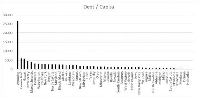
The top five states for debt per capita were Wyoming, Connecticut, Hawaii, New Jersey and Massachusetts in descending order. The bottom five states were Oklahoma, Tennessee, Montana, Indiana and Nebraska in descending order. Only Nebraska, which had the smallest amount of debt per capita, was also in the top five states for financial condition. Interestingly, Wyoming which had the second highest financial condition also had the highest amount of debt per capita. See figure 2.
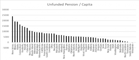
The top five states for unfunded state pensions per capita were New Jersey, Illinois, Alaska, Connecticut and Kentucky in descending order. The bottom five states were Delaware, North Carolina, Tennessee, South Dakota and Wisconsin in descending order. Here the picture is clearer; Most of the states in the top five for unfunded pensions also have the lowest financial condition. This includes Illinois, New Jersey, Connecticut and Kentucky. See figure 3.
In order to better understand these relationships, I did a bootstrapped multiple regression to account for the small sample size (N = 50 states). The outcome variable was financial condition while debt per capita and unfunded pensions per capita were predictor variables. A number of control variables were included in the regression as well including Medicaid spending per enrollee, GDP in current dollars, intergovernmental aid, state population, unemployment, median household income, Federal Matching Rate for Medicaid, the housing price index and the Census region.
Figure 1: Averaged State Financial Condition
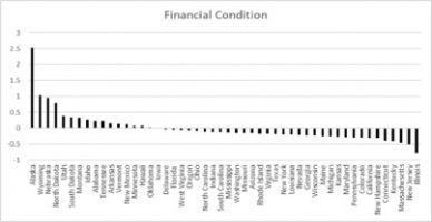
Figure 2: Averaged Debt per Capita
Based on the results of the regression, debt per capita was not a significant predictor of state financial condition. This was expected given the lack of linearity between these variables. However, the effect was in the expected direction. The unfunded pensions per capita was a significant predictor of financial condition. The effect was negative as expected. This means that an increase in the amount of unfunded pensions per capita decreases the financial condition in a state. See table 1 (only these variables are shown there).
Figure 3: Averaged Unfunded Pensions per Capita
|
Table 1: Regression Results
|
|
Variables
|
Β(β)
|
Std. Error
|
|
Unfunded Pension / Capita
|
-.000016 (-.167)*
|
.0000002
|
| |
(-.0000164, -.0000158)
|
|
|
Debt / Capita
|
-.000000126 (-.001)
|
.0000002
|
| |
(-.0000005, .00000025)
|
|
|
Notes. Sample bootstrapped 5000 times (N = 252550). Confidence intervals bias-corrected and accelerated (95% confidence interval). Df = 252539. *ρ ≤ .0001. R2 = .617. F ratio = 36971 (ρ ≤ .0001).
|
The interpretation of these findings is that although the amount of debt a state had had a negative effect on state financial condition, it did not matter as much as the unfunded pension amount. It is not new information that states and local governments have struggled with paying their pension obligations. This analysis shows that between 2006 and 2017 it was a significant predictor of financial condition. What is not addressed in this analysis is what states can do to close these gaps. More research is needed to understand these dynamics.
Author: Dr. Hummel is an assistant professor in the Department of Philanthropy, Nonprofit Leadership and Public Affairs at Slippery Rock University. He teaches classes on civic engagement, leadership and financial decision making. His email is [email protected]. You can also visit his website: www.hummel-research.com.
 (No Ratings Yet)
 Loading...

State Financial Condition in The United States The Last Ten Years
The views expressed are those of the author and do not necessarily reflect the views of ASPA as an organization.
By Daniel Hummel
November 23, 2019
In the tumultuous years between 2006 and 2017 there had been much change in the United States. We had three different presidents, the Great Recession and one major change to healthcare (The Affordable Care Act). It was also a time of change for state budgets. Recently, I averaged a financial condition measure for the fifty states across the years 2006, 2010, 2014, 2016 and 2017 for a project. I chose these years based on their proximity to the Great Recession and some milestones with the implementation of the Affordable Care Act. I used the financial condition measure designed by Wang, Dennis and Tu which sums up a series of standardized and weighted ratios based on short-term and long-term financial variables. This data is available in state financial reports. I used equal weightings as advised by Norcross and Gonzalez at the Mercatus Center which also uses this measure to rank the states.
The top five states were Alaska, Wyoming, Nebraska, North Dakota and Utah in descending order. The bottom five states were Connecticut, Kentucky, Massachusetts, New Jersey and Illinois in descending order. See figure 1. In order to understand why these states had the financial condition they did during this time period I looked at two commonly identified factors for financial condition, debt held by the state per capita and the amount of unfunded state pensions per capita. I was able to acquire the debt data from the state financial reports. The Mercatus Center had collected the data on unfunded pensions until 2016 and Dr. Joshua Rauh of Stanford University published the data for 2017 on his website. These were averaged across the same years as the financial condition measure.
The top five states for debt per capita were Wyoming, Connecticut, Hawaii, New Jersey and Massachusetts in descending order. The bottom five states were Oklahoma, Tennessee, Montana, Indiana and Nebraska in descending order. Only Nebraska, which had the smallest amount of debt per capita, was also in the top five states for financial condition. Interestingly, Wyoming which had the second highest financial condition also had the highest amount of debt per capita. See figure 2.
The top five states for unfunded state pensions per capita were New Jersey, Illinois, Alaska, Connecticut and Kentucky in descending order. The bottom five states were Delaware, North Carolina, Tennessee, South Dakota and Wisconsin in descending order. Here the picture is clearer; Most of the states in the top five for unfunded pensions also have the lowest financial condition. This includes Illinois, New Jersey, Connecticut and Kentucky. See figure 3.
In order to better understand these relationships, I did a bootstrapped multiple regression to account for the small sample size (N = 50 states). The outcome variable was financial condition while debt per capita and unfunded pensions per capita were predictor variables. A number of control variables were included in the regression as well including Medicaid spending per enrollee, GDP in current dollars, intergovernmental aid, state population, unemployment, median household income, Federal Matching Rate for Medicaid, the housing price index and the Census region.
Figure 1: Averaged State Financial Condition
Figure 2: Averaged Debt per Capita
Based on the results of the regression, debt per capita was not a significant predictor of state financial condition. This was expected given the lack of linearity between these variables. However, the effect was in the expected direction. The unfunded pensions per capita was a significant predictor of financial condition. The effect was negative as expected. This means that an increase in the amount of unfunded pensions per capita decreases the financial condition in a state. See table 1 (only these variables are shown there).
Figure 3: Averaged Unfunded Pensions per Capita
Table 1: Regression Results
Variables
Β(β)
Std. Error
Unfunded Pension / Capita
-.000016 (-.167)*
.0000002
(-.0000164, -.0000158)
Debt / Capita
-.000000126 (-.001)
.0000002
(-.0000005, .00000025)
Notes. Sample bootstrapped 5000 times (N = 252550). Confidence intervals bias-corrected and accelerated (95% confidence interval). Df = 252539. *ρ ≤ .0001. R2 = .617. F ratio = 36971 (ρ ≤ .0001).
The interpretation of these findings is that although the amount of debt a state had had a negative effect on state financial condition, it did not matter as much as the unfunded pension amount. It is not new information that states and local governments have struggled with paying their pension obligations. This analysis shows that between 2006 and 2017 it was a significant predictor of financial condition. What is not addressed in this analysis is what states can do to close these gaps. More research is needed to understand these dynamics.
Author: Dr. Hummel is an assistant professor in the Department of Philanthropy, Nonprofit Leadership and Public Affairs at Slippery Rock University. He teaches classes on civic engagement, leadership and financial decision making. His email is [email protected]. You can also visit his website: www.hummel-research.com.
Follow Us!